Jeff Kabachinski
This installment of Networking looks into network bridging, specifically a type of bridge called a filtering bridge and the process by which it makes packet-forwarding decisions. We’ll examine this main bridging premise and how bridges can segment network traffic. Since network switches can be thought of as multiport bridges, understanding fundamental bridge function also means understanding fundamental switch function.
Bridges and switches operate at layer 2 (data link layer) of the OSI Reference Model, the local area network (LAN) layer. Ethernet also functions at layer 2. The term bridge is also used for some layer 1 devices that simply forward all packets, like a repeater or hub. (The use of network terminology can be arbitrary in that the terms are mixed and used interchangeably all the time. When talking about networking, be aware of the context in which terms are used—you may need to translate to ensure understanding!)
The data link layer has two sub-layers, the media access control (MAC) and the logical link control (LLC). The LLC is a protocol defined by IEEE 802.2 that arbitrates for network node access to send packets. It uses the MAC sub-layer that defines the unique hard coded MAC level address. This is why the Ethernet address is often referred to as the MAC address.
Ethernet Addressing
The Ethernet address is integral to how bridges operate. The first pieces of information in an Ethernet packet are the relative Ethernet addresses. The destination address comes first in the packet, identifying the network node the packet is intended for. The second address in the packet is the source address, indicating who sent it.
Ethernet addresses are six bytes in length. Each byte is written in hexadecimal format where bytes are delimited by a colon. An example could be 00:00:A1:FD:23:C9, perhaps as a destination address of the intended recipient. This is immediately followed by the source address or the address of the sender. The source address would obviously be different that the destination address.
The Ethernet Envelope
The Ethernet envelope is not dissimilar from our human protocol for snail mail. We use the upper left corner of the front of the envelope for the from or source address identifying the sender. Somewhere near the middle of the front of the envelope we put the to or destination address identifying the intended recipient. Upon receipt we look to see if it’s our name and address before opening. If not—we’ll toss it aside.
You can think of the Ethernet packet as an envelope where the header and delivery information is on the outside of the envelope and the data payload is inside the envelope. The Ethernet circuitry in each network node grabs a copy of every LAN packet going by on the wire. It then examines the packet for the destination address, accepting packets with its own address and tossing aside all other traffic. An Ethernet address is unique for each LAN node and is known as the unicast address. There also is a broadcast address, which is another packet that all nodes accept. The broadcast Ethernet address is easily recognizable—all digital ones, or FF:FF:FF:FF:FF:FF. For the human analogy, a broadcast address might be Resident or Occupant.
Upon receipt of the data packet, the Ethernet circuitry looks to see if it recognizes its own unicast address (or broadcast address) as the destination. If it does, it accepts the packet. If not, the circuitry will throw the data packet away. If it is a unicast address, the Ethernet circuitry also checks the source address to see who sent it. The Ethernet circuitry then performs a checksum analysis to verify that the packet arrived intact before extracting the data payload and forwarding it upstream.
The Self-Learning Function
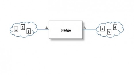
Figure 1. The basic bridge.
Consider the bridge depicted in Figure 1. The two clouds shown represent two LANs. For demonstration purposes, we can see nodes 1, 2, and 3 in one cloud, and nodes 4, 5, and 6 in the other. Bridges are smart. In other words, they are equipped with a CPU using specific bridge programming. The bridge pulls in every data packet that it senses on the cable and reads the Ethernet addressing information.
For each packet that comes in on the A side, the bridge reads and remembers the source address from the packet. After a few hundred milliseconds or so, the bridge will have a list of all the source addresses it hears on segment A. Now the bridge knows the Ethernet addresses of all the nodes communicating on segment A. The same self-learning cycle happens on the B side, creating a list of the Ethernet addresses of the nodes on the B LAN by listening in on the data packets and keeping track of the source addresses. This is where the bridging tables come from, and they are used for subsequent bridging decisions. Over time bridges will also intermittently send broadcasts asking for a reply, in order to keep its address lists up to date.
As an example, node 2 is attempting to communicate with node 3 in Figure 1. The bridge would sense and read this packet and know from its addressing tables that node 2 and node 3 are on LAN A. It recognizes that there is no need to send that packet to LAN B, since the nodes out there will just throw it away. Thus the bridge is up and that packet will not be sent over to LAN B. This also cuts down on extraneous network traffic on LAN B.
However, if node 3 is in communication with node 4, the bridge would recognize that node 4—the destination—is on the B side. Therefore, it lowers the bridge and passes that data packet through.
The main premise of bridging described here is called a filtering bridge. Filtering bridges are self-learning, using the Spanning Tree Protocol (STP) defined in the IEEE 802.1 standard. STP can also be used for other bridges on the network to detect and manage redundant links. Obviously, once a CPU is in the picture, programming can start to include more options and function like this. For example, a degree of security can be employed by denying access to a “secured LAN port” to all requesting network nodes that do not have their MAC address on the secured LAN’s network node access list maintained in the bridge. Finally, a switch can be thought of as a multiport bridge, in essence. By adding a few more LAN segments to the bridge shown in Figure 1, our self-learning bridge will forward packets only to the LAN where the intended recipient resides.
Summary
A bridge is smart. It reads the Ethernet packets and checks on the addressing. The bridge builds a list of all the source addresses it senses on each LAN connection, and doesn’t take long to build these address tables. When it sees a packet where the source and destination address are on the same table, it knows to draw the bridge up. It will lower it only for traffic that needs to pass through to the other side, based on Ethernet addressing. In addition, when a bridge encounters a badly formed or corrupted packet it will just throw it away, helping to minimize unnecessary network traffic.
For more information on network bridges, be sure to scan the standards. See IEEE 802.1 for the Spanning Tree Protocol, IEEE 802.2 for the logical link control, and IEEE 802.3 for Ethernet. 24×7
Jeff Kabachinski is the director of technical development for Aramark Healthcare Technologies in Charlotte, NC. For more information, contact [email protected].